
Empirical Exercise 3
In this exercise, we’re going to analyze data from Ignaz Semmelweis’ handwashing intervention in the maternity hospital in Vienna. The data come from Semmelweis’ (1861) book, and some helpful person put them on Wikipedia.
We’ll review the different ways to estimate simple difference-in-differences models. We’ll also learn how to make simple graphs using twoway and export regression results using the esttab and putexcel commands. putexcel is more customizable, but it also takes more work. esttab is a very straightforward tool for getting basic regression results out of stata and into pretty much any format.
Additional tips on using Stata for data visualization are available here. Tips on making tables are available here.
Getting Started
Data on maternal mortality rates in Vienna are contained in the Excel file E3-Semmelweis1861-data.xlsx. The spreadsheet inlcudes annual data from 1833 (when the Vienna Maternity Hospital opened its second clinic) through 1858. Mortality rates are reported for Division 1 (where expectant mothers were treated by doctors and medical students) and Division 2 (where expectant mothers were treated by midwives and trainee midwives from 1841 on). In Semmelweis’ difference-in-differences analysis, Division 1 was the (ever-)treated group.
Our first task is to import this Excel file into Stata using the import excel command. Create a do file that begins with the usual
preliminaries and then imports the Semmelweis data directly from github using the following code:
import excel ///
"https://pjakiela.github.io/ECON523/exercises/E3-Semmelweis1861-data.xlsx", ///
sheet("ViennaBothClinics") first
The option sheet tells Stata which worksheet within the excel file E3-Semmelweis1861-data.xlsx to select. The option first indicates that the first row of the spreadsheet should be treated as variable names and not as one of the observations.
After importing the data, assign the variables the following labels using the label var command:
| Variable | Label to Assign |
|---|---|
| Births1 | Births in Division 1 (Treatment Group) |
| Deaths1 | Deaths in Division 1 (Treatment Group) |
| Rate1 | Mortality Rate in Division 1 (Treatment Group) |
| Births2 | Births in Division 2 (Comparison Group) |
| Deaths2 | Deaths in Division 2 (Comparison Group) |
| Rate2 | Mortality Rate in Division 2 (Comparison Group) |
Now familiarize yourself with the data set. What is the average maternal mortality rate in Division 1? What is the average maternal mortality rate in Division 2?
In-Class Activity
Question 1
Use stata’s twoway command to make a graph of maternal mortality in the two wings of the hospital. First, if you have not already, install the blindschemes packing by running the command:
ssc install blindschemes
This will allow you to use the colors sea and vermillion from the Okabe-Ito colorblind-friendly palette, as shown in the sample code. Adapt the code to make your graph as close possible to the one below.
twoway (connected Rate1 Year, ///
	color(vermillion) msymbol(o) msize(small) lw(thin)) ///
	(connected Rate2 Year, ///
	color(sea) msymbol(o) msize(small) lw(thin)), ///
	xlabel(1830(5)1860) xtitle(" ") ///
	legend(label(1 "Doctors' Wing") ///
	label(2 "Midwives' Wing") ///
	col(2) ring(0) pos(2))
Your finished graph should look something like this:
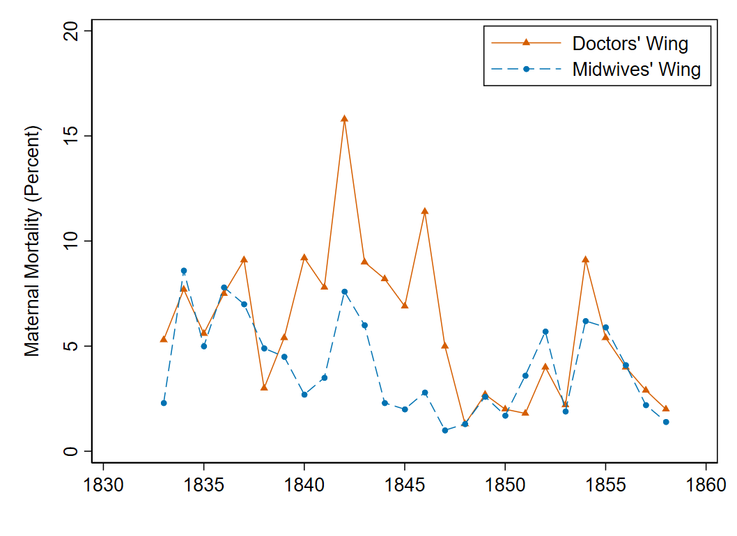
What patterns do you notice in this figure? How do maternal mortality rates in the two divisions of the hospital compare?
Question 2
In what year did the hospital first move to the system where patients in Division 1 were treated by doctors and patients in Division 2 were treated by midwives? Drop the observations (years) before this happened using the drop command.
Hint: use the list command to list the the notes contained in the data set by year. If you only want to list the rows of data that include a note (i.e. where the Note variable is non-missing), you can add !missing(Note) at the end of the command.
Question 3
Generate a post variable equal to one for years after the handwashing policy was implemented (and zero otherwise).
Question 4
What is the mean postpartum mortality rate in the doctors’ wing (Division 1) prior to the implementation of the handwashing policy?
Question 5
Now we’re going make a table showing the difference-in-differences estimate of the treatment effect of hand washing on maternal mortality. The table will show the mean mortality rate (maternal deaths per 100 births) in the Treatment and Comparison wings before and after Semmelweis’ policy was implemented. Your table will look something like this, except with the actual means, standard errors, and differences instead of ones and zeroes:
| Treatment | Comparison | Difference | |
|---|---|---|---|
| Before Handwashing | 1.00 | 1.00 | 1.00 |
| (0.00) | (0.00) | (0.00) | |
| After Handwashing | 1.00 | 1.00 | 1.00 |
| (0.00) | (0.00) | (0.00) | |
| Difference | 1.00 | 1.00 | 1.00 |
| (0.00) | (0.00) | (0.00) |
We’ll write to an excel file using the putexcel command . putexcel is a simple command that allows you to write Stata output to a particular cell or set of cells in an excel file. Before getting started with putexcel, use the pwd (“print working directory”) command to make sure that you are writing your results to an appropriate folder. Use cd to change your file path if necessary. Then set up the excel file that will receive your results using the commands:
putexcel set E3-DD-table1.xlsx, replace
putexcel B1="Treatment", hcenter bold border(top)
putexcel C1="Comparison", hcenter bold border(top)
putexcel D1="Difference", hcenter bold border(top)
putexcel A2="Before Handwashing", bold
putexcel A4="After Handwashing", bold
You will also want to set the widths of the columns in your Excel file. Unfortunately, there is no way to do this using putexcel. The code below invokes stata’s mata programming language to adjust the column widths. Change the parameter values as needed to create a professional-looking table.
mata
b = xl()
b.load_book("E3-DD-table1.xlsx")
b.set_sheet("Sheet1")
// make variable name column widest
b.set_column_width(1,1,20)
// width for subsequent columns
b.set_column_width(2,4,12)
// row heights
b.set_row_height(2,7,20)
b.set_row_height(2,7,20)
// make headers bold
cols = (1,4)
b.set_font_bold(1, cols, "on")
// top and bottom borders
b.set_bottom_border(7, cols, "thin")
b.set_top_border(1, cols, "thin")
b.set_top_border(2, cols, "thin")
b.close_book()
end
At this point, it is worth opening your excel file to make sure that you are writing to it successfully. Be sure to close the file after you look at it; Stata won’t write over an open file. The column and row labels should all appear in bold font; the column headings in cells B1, C1, and D1 should be centered; and the table should have borders at the top and bottom.
Question 6
Now that we know that putexcel is working, we can add the mean of the variable Rate1 (the maternal mortality rate in Division 1) for the years prior to the introduction of handwashing. You can use the return list command after a command like summarize to see what statistics the summarize command stored in Stata’s short-term memory as locals. Any of these statistics can be exported to Excel.
sum Rate1 if post==0
return list
We’re going to put the mean maternal mortality rate in Division 1 prior to the handwashing intervention in cell B2: the Treatment column, in the Before Handwashing row.
local temp_mean = string(r(mean),"%03.2f")
putexcel B2=`temp_mean', hcenter
The string command in the first line creates a local macro containing a string that is the mean calculated the last time you used the summarize command, rounded to 2 decimal places. The second line writes that local macro in our Excel file. Notice that the local macro being exported to Excel appears in single quotes. If you are just writing a local macro to Excel using the putexcel command, it does not need to appear in (double) quotes, but sequences of letters and numbers do need double quotes. The hcenter option tells Excel to center the number within the column.
Question 7
We can calculate the standard error of the mean by taking the standard deviation (reported by the sum command) and dividing it by the square root of the number of observations (also reported by the sum command). What is the standard error of the mean postpartum mortality rate in the doctors’ wing prior to Semmelweis’ handwashing intervention? Use the code below to add this to your table.
local temp_se = string(r(sd)/sqrt(r(N)),"%03.2f")
putexcel B3="(`temp_se')", hcenter
Question 8
We can also use the ci means command to calculate the mean and standard error of a variable. Use
return list to see what statistics are saved after ci means. Use ci means and putexcel to add
the mean and standard error of Rate1 in the post-treatment period to your table.
Question 9
Calculate the difference (between the mean of Rate1 in the pre-treatment period and the mean of Rate1 in the post-treatment period) and the associated standard error by hand using the formula (and the display command).
Question 10
Now confirm that you get the same result using the ttest command. How would you export the results of the ttest command into your table using putexcel?
Question 11
Now complete the table.
Empirical Exercise
Next, we are going to implement difference-in-differences as a regression. Create a do file that reads in Semmelweis’ data from github and restricts attention to the period when doctors worked in the first clinic and midwives worked in the second clinic. Your do file should start with the usual preliminaries, just like your do file for the in-class activity.
Question 1
Generate a post variable equal to one for years after the handwashing policy was implemented (and zero otherwise), and then generate a diff variable equal to the difference in mortality rates between Clinic 1 (treatment) and clinic 2 (control). Regress diff on post. Use the command eststo clear immediately before your regression command, and then use the command eststo (short for “estimates store”) immediately after. This will save your regression results. Then display your results with esttab with the se (standard error) option (esttab, se). What is the coefficient on post, which is the difference-in-difference-in-differences estimate of the treatment effect of handwashing? What is the associated standard error? What is the t-statistic?
Question 2
Use the reshape command (illustrated below) to convert your data into a panel data set containing a variable Rate and a variable clinic that indicates whether an observation comes from Clinic 1 (doctors) or Clinic 2 (midwives). How many observations are there in the data set now? How many from each clinic?
reshape long Rate, j(clinic) i(Year)
Question 3
Generate a treatment variable equal to one for the doctors’ wing (and zero otherwise). Then generate the interaction term you need to estimate a difference-in-differences model in a regression framework.
Question 4
Use the label variable command to give your variables short, easy to interpret labels. I suggest the following:
| Variable | Label to Assign |
|---|---|
| treatment | Treatment clinic |
| post | Handwashing implemented (post) |
| txpost | Treatment*post |
Question 5
Implement (standard 2x2) difference-in-differences in an OLS regression framework. Use the command eststo clear immediately before your regression command, and then use the command eststo (estimates store) to save your results. What is the coefficient on your txpost (treatment x post) variable? what is the standard error?
Question 6
Now implement differences in differences while controlling for year fixed effects: omit the post variable from your regression, and instead include i.Year to generate and include year fixed effects. Use eststo to store your results (do not use eststo clear first because you want to store the results from both regressions). What is the coefficient on your txpost variable? what is the standard error? Did including fixed effects improve the precision of your estimates?
Question 7
Use the esttab command to make a table of your regression results, and then use esttab using clinic-regs.rtf to save your table as a word (rtf) document. Look through the esttab options to make your table look more professional. Report standard errors rather than t-statistics in parentheses below your coefficients. Have your variable labels appear in place of variable names, and make sure your first column is wide enough to accommodate the labels you have given your variables. Make the columns with your regression coefficients say OLS at the top using esttab’s mtitle option. Adding indicate(Year Fixed Effects = *.Year) will tell esttab to omit the coefficients on the fixed effects and instead indicate where they are included. You can learn more about making tables in esttab here. Export your finished table to word and then save it as a pdf so that you can upload it to gradescope.
Optional. If you want to make a fully customizable table using putexcel, you can instead run your regressions, store the results in new stata variables that you create, and export those to excel, as follows:
reg Rate treatment post txpost
mat V = r(table)
mat list V
You see that you have your regression results stored in the matrix V. You could use putexcel to write those results one coefficient at a time, or you could create the column of results that you want in your table as a variable and then export it, like this:
gen results = ""
replace results = string(V[1,1],"%03.2f") in 1
replace results = string(V[2,1],"%03.2f") in 2
replace results = string(V[1,2],"%03.2f") in 3
replace results = string(V[2,2],"%03.2f") in 4
replace results = string(V[1,3],"%03.2f") in 5
replace results = string(V[2,3],"%03.2f") in 6
replace results = string(V[1,4],"%03.2f") in 7
replace results = string(V[2,4],"%03.2f") in 8
replace results = "(" + results + ")" if mod(_n,2)==0 & results!=""
putexcel set E3-DD-regs.xlsx, replace
putexcel B1="(1)", hcenter bold border(top)
putexcel B2="OLS", hcenter bold border(bottom)
export excel results using E3-DD-regs.xlsx, cell(B3) sheet("Sheet1", modify)
Extend the code so that you end up with a nicely formatted regression table containing the results of both regressions, complete with variable labels, borders, etc. You can also use a similar approach to export your results to latex, if you prefer.
Question 8
When you upload your do file to gradescope, you will be asked to answer the following questions about your results:
- Which coefficient in the regression table (i.e. the coefficient on which variable) is the difference-in-differences estimate of the treatment effect of handwashing on maternal mortalty?
- Which regression coefficient is the estimate of the degree of selection bias?
- Which regression coefficient is the estimate of the time trend in the absence of treatment?
- In one sentence, explain how adding fixed effects changed the precision of your difference-in-difference estimate of the impact of handwashing.
This exercise is part of Module 3: Difference-in-Differences 1.