Empirical Exercise 3 in R

In this exercise, we’re going to analyze data from Ignaz Semmelweis’ handwashing intervention in the maternity hospital in Vienna. The data come from Semmelweis’ (1861) book, and some helpful person put them on Wikipedia.

We’ll review the different ways to estimate simple difference-in-differences models. We’ll also learn how to make simple graphs using ggplot and export regression results to excel using openxls.

Getting Started

Data on maternal mortality rates in Vienna are contained in the Excel file E3-Semmelweis1861-data.xlsx. The spreadsheet inlcudes annual data from 1833 (when the Vienna Maternity Hospital opened its second clinic) through 1858. Mortality rates are reported for Division 1 (where expectant mothers were treated by doctors and medical students) and Division 2 (where expectant mothers were treated by midwives and trainee midwives from 1841 on). In Semmelweis’ difference-in-differences analysis, Division 1 was the (ever-)treated group.

Our first task is to import this Excel file into R using the openxlsx package. Create R script that begins with the usual preliminaries, installs the package openxlsx and loads it as one of the libraries, and then imports the Semmelweis data directly from github using the following code:

url <- "https://pjakiela.github.io/ECON523/exercises/E3-Semmelweis1861-data.xlsx"
e3data <- tibble(read.xlsx(url, sheet = "ViennaBothClinics"))

The option sheet tells R which worksheet within the excel file E3-Semmelweis1861-data.xlsx to select. After importing the data, you should observe the following columns in the e3data data frame:

Columns	Description
Births1	Births in Division 1 (Treatment Group)
Deaths1	Deaths in Division 1 (Treatment Group)
Rate1	Mortality Rate in Division 1 (Treatment Group)
Births2	Births in Division 2 (Comparison Group)
Deaths2	Deaths in Division 2 (Comparison Group)
Rate2	Mortality Rate in Division 2 (Comparison Group)

Now familiarize yourself with the data set. What is the average maternal mortality rate in Division 1? What is the average maternal mortality rate in Division 2?

In-Class Activity

Question 1

Use R’s ggplot package to make a graph of maternal mortality in the two wings of the hospital. First, use the following code to define the dark blue and dark orange color’s from the Okabe-Ito colorblind-friendly palette

oiblue <- "#0072B2"
oiverm <- "#D55E00"

This will allow you to use the colors oiblue and oiverm, as shown in the sample code. Adapt the code to make your graph as possible to the one below.

ggplot(e3data, aes(x = Year, y = Rate1)) + 
  geom_point(color = oiblue, shape = 16, size = 0.8) +
  geom_line(aes(color = 'Doctors'), linewidth = 0.32) +
  geom_point(aes(y = Rate2), color = oiblue, shape = 16, size = 0.8) +
  geom_line(aes(y = Rate2, color = 'Midwives'), linewidth = 0.32) +
  xlab(" ") +
  ylab("Maternal Mortality (Percent)") + 
  scale_x_continuous(n.breaks=6) +
  scale_color_manual(name=' ',
                     breaks=c('Doctors',
                              'Midwives'),
                     values=c('Doctors' = oiverm,
                              'Midwives' = oiblue)) 

Your finished graph should look something like this: all-data-plot

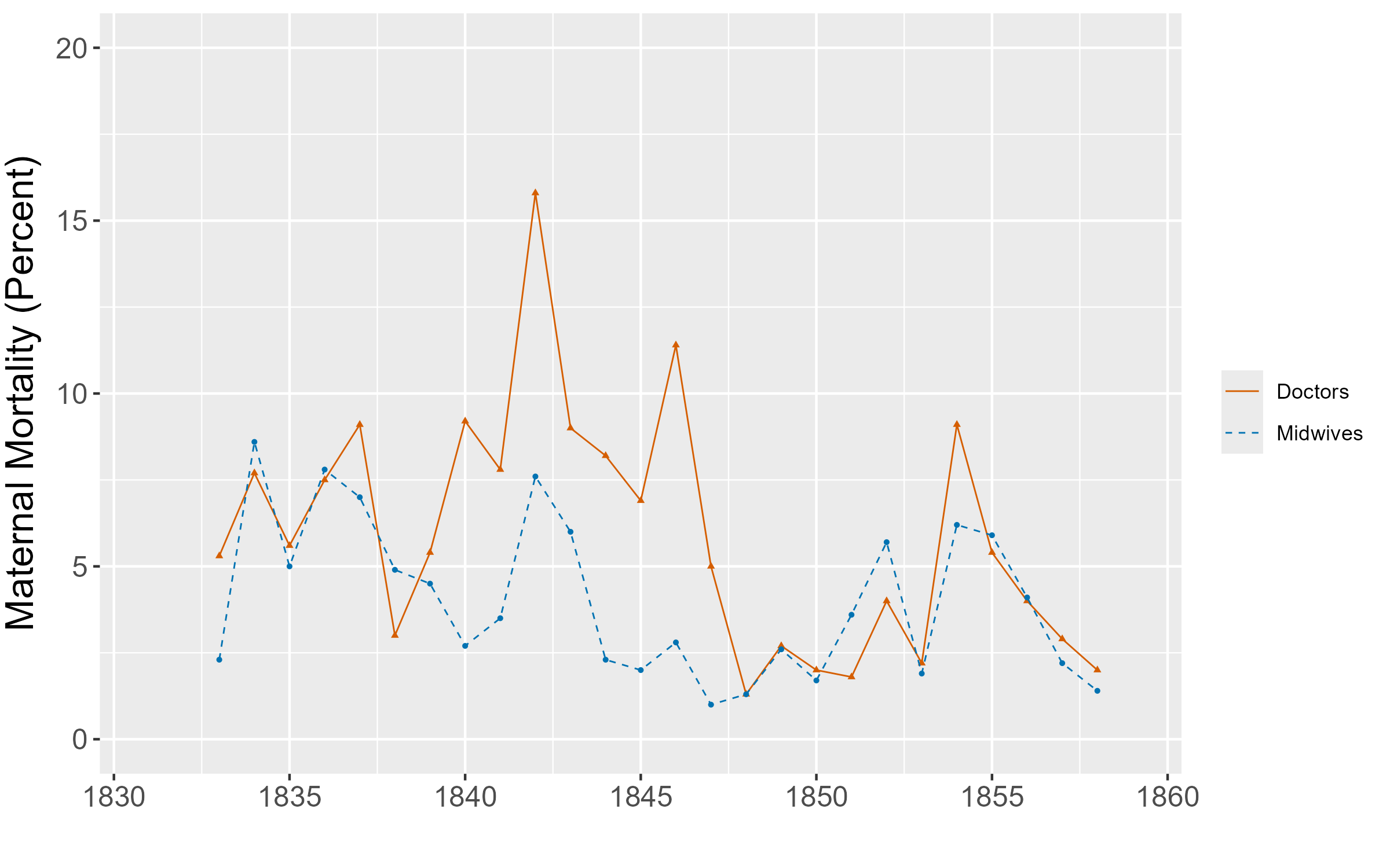
What patterns do you notice in this figure? How do maternal mortality rates in the two divisions of the hospital compare?

Question 2

In what year did the hospital first move to the system where patients in Division 1 were treated by doctors and patients in Division 2 were treated by midwives? Drop the observations (years) before this happened.

Hint: use print(df, n = 100) to print the first 100 rows of data frame df. Then use select() to keep the correct rows.

Question 3

Generate a post variable equal to one for years after the handwashing policy was implemented (and zero otherwise).

Question 4

What is the mean postpartum mortality rate in the doctors’ wing (Division 1) prior to the implementation of the handwashing policy?

Question 5

Now we’re going make a table showing the difference-in-differences estimate of the treatment effect of hand washing on maternal mortality. The table will show the mean mortality rate (maternal deaths per 100 births) in the Treatment and Comparison wings before and after Semmelweis’ policy was implemented. Your table will look something like this, except with the actual means, standard errors, and differences instead of ones and zeroes:

	Treatment	Comparison	Difference
Before Handwashing	1.00	1.00	1.00
	(0.00)	(0.00)	(0.00)
After Handwashing	1.00	1.00	1.00
	(0.00)	(0.00)	(0.00)
Difference	1.00	1.00	1.00
	(0.00)	(0.00)	(0.00)

We’ll write to an excel file using openxlsx saveWorkbook(), a simple command that allows you to write a data frame to an excel file. Before getting started with saveWorkbook(), we will define a simple data frame that contains our desired column and row headings as well as placeholders for the results we want to report. Use the code below to do this. Notice that the second, third, and fourth columns of the tibble that we create are named Treatment, Comparison, and Difference.

labels <- c("Before Handwashing", 
            " ", 
            "After Handwashing", 
            " ", 
            "Difference", 
            " ")
temp_column <- c("11", "00", "11", "00", "11", "00")
e3_results <- tibble(" " = labels, 
                     "Treatment" = temp_column, 
                     "Comparison" = temp_column, 
                     "Difference" = temp_column)
print(e3_results)

Now we use createWorkbook(), addWorksheet(), writeData(), and saveWorkbook() to write the data frame e3_results to excel. In addition to those key steps, the code below uses setColWidths() and addStyle() to format the table. Adjust the formatting parameters as desired.

wb <- createWorkbook()
addWorksheet(wb, "Results")
# create a header style
hs1 <- createStyle(halign = "CENTER", textDecoration = "Bold", border = "BottomTop")
# write the results to the table
writeData(wb, "Results", e3_results, headerStyle = hs1)
# adjust column widths
e3_widths <- c(18, 12, 12, 12)
setColWidths(wb, "Results", cols = 1:4, widths = e3_widths)
# center the content of the table
center_style <- createStyle(halign = "CENTER")
addStyle(wb, "Results", center_style, cols = 2:4, rows = 1:7, gridExpand = TRUE, stack = TRUE)
# create a bottom border
bottom_style <- createStyle(border = "Bottom")
addStyle(wb, "Results", bottom_style, cols = 1:4, rows = 7, gridExpand = TRUE, stack = TRUE)
# save workbook
saveWorkbook(wb, file = paste0(pjpath, "/R3-DD1.xlsx"), overwrite = TRUE)

At this point, it is worth opening your excel file to make sure that you are writing to it successfully. Be sure to close the file after you look at it; R won’t write over an open excel file. The column labels should all appear in bold font, and there should be borders at the top and bottom of the table.

Question 6

Now that we know the openxls commands are working, we can add the mean of the variable Rate1 for the years prior to the introduction of handwashing. Calculate the mean, and then use as.character() to convert it to a string that you call pre_mean_1. You can use df[rownum, colnum] to index a particular cell in a data frame. Update the data frame e3_results by replacing the appropriate cell with pre_mean_1, as illustrated in the code below. Then re-run the code that creates your excel workbook to see that you have successfully exported your first result.

pre_mean_1 <- as.character(mean(dd_data$Rate1[dd_data$Year <= 1846]))
e3_results[1, 2] <- pre_mean_1

Question 7

You can complete the table by calculating each statistic individually, but it is easier and faster to manipulate the data as a matrix. The code below uses group_by() and summarize() to calculate the mean, SD, and number of observations for Rate1 and Rate2 in the pre-treatment and post-treatment periods, and then calculates the standard error of the mean of Rate1 as well as the standard error of the difference in means between Rate1 and Rate2. Extend the code so that you also calculate the standard error of the mean of Rate2, and then drop the columns containing the SDs and Ns from the data frame.

ddresults <- e3data %>% 
  select(Rate1, Rate2, post) %>% 
  group_by(post) %>% 
  summarise(across(where(is.numeric), .fns = 
                                        list(mean = mean,
                                             sd = sd,
                                             n = ~ n()
                                        ))) %>% 
  mutate(Rate1_se = Rate1_sd / sqrt(Rate1_n), 
         diff = Rate1_mean - Rate2_mean, 
         diff_se = sqrt(Rate1_se ** 2 + Rate2_se ** 2)) 

Question 8

We now have a data frame ``ddresults that contains six columns: three means and three standard errors. We want to create a data frame that displays the standard errors below the means. To do this, start by creating separate data frames ddresults_mean and ddresults_se that select the appropriate columns from ddresults`.

Question 9

The code below illustrates how we can add an additional row to ddresults_se containing the standard errors of the differences in means (pre v.s post). Implement a similar procedure to add a row containing the difference in means (pre vs. post) to the ddresults_mean data frame.

pre_vs_post_se <- ddresults_se[1, ] ** 2 + ddresults_se[2, ] ** 2
pre_vs_post_se <- sqrt( pre_vs_post_se)
ddresults_se <- rbind(ddresults_se, pre_vs_post_se)

Question 10

Before we export our results to excel, we need to format them appropriately and convert them to strings. The code below shows how to do this for the standard errors contained in ddresults_se, and then illustrates how we can transfer our standard errors to the e3_results data frame that we intend to export to excel. Extend the code so that you also include the appropriately-formatted means in e3_results. Then, print e3_results to make sure that you are ready to write your findings to excel.

ddresults_se <- ddresults_se %>% 
  mutate(across(1:3, ~ sprintf("%.2f", .))) %>% 
  mutate(across(everything(), as.character)) %>% 
  mutate(across(everything(), ~ str_c("(", ., ")")))
e3_results[2, 2:4] <- ddresults_se[1, ]
e3_results[4, 2:4] <- ddresults_se[2, ]
e3_results[6, 2:4] <- ddresults_se[3, ]

Question 11

Now export e3_results to excel, adapting the code from Question 5. Make sure that your code now produces a correct, correctly-formatted table showing the difference-in-differences estimate of the impact of handwashing on maternal mortality.

Empirical Exercise

Next, we are going to implement difference-in-differences as a regression. Create a new R script file that reads in Semmelweis’ data from github and restricts attention to the period when doctors worked in the first clinic and midwives worked in the second clinic. Your script should start with the usual preliminaries, just like the one you wrote for the in-class activity.

Question 1

Use pivot_longer() (illustrated below) to convert your data into a panel data set containing a variable Rate and a variable clinic that indicates whether an observation comes from Clinic 1 (doctors) or Clinic 2 (midwives). How many observations are there in the data set now? How many from each clinic?

e3panel <- e3data %>% 
  pivot_longer(!Year, names_to = "clinic", values_to = "Rate") %>% 
  mutate(clinic = if_else(clinic == "Rate1", "1", "2"))
dim(e3panel)

Question 2

Generate a post variable equal to one for years after the handwashing policy was implemented (and zero otherwise) and a treatment variable equal to one for the doctors’ wing (and zero otherwise).

Question 3

Generate the interaction term you need to estimate a difference-in-differences model in a regression framework.

Question 4

Implement difference-in-differences in an OLS regression framework. Store your results.

Question 5

The code below will create a data frame containing the coefficients and standard errors from your regression. Adapt the code from the In-Class Activity to format the values (rounding them to two or three decimal places and then converting them to strings).

results <- model$coeftable[,1:2]

Question 6

Modify the results data frame so that it is ready to be exported to excel. You are free to leave the coefficients and standard errors in separate columns if you wish, but make sure to add well-formatted labels for the rows and clean up the column names.

Question 7

Adapt the code from the In-Class Activity to export your regression results to excel.

Question 8

When you upload your code and excel file to gradescope, you will be asked to answer the following questions about your results:

Which coefficient in the regression table (i.e. the coefficient on which variable) is the difference-in-differences estimate of the treatment effect of handwashing on maternal mortalty?
Which regression coefficient is the estimate of the degree of selection bias?
Which regression coefficient is the estimate of the time trend in the absence of treatment?

This exercise is part of Module 3: Difference-in-Differences 1.