Empirical Exercise 4

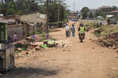
In this exercise, we’re going to replicate the difference-in-differences analysis from Does a ban on informal health providers save lives? Evidence from Malawi by Professor Susan Godlonton and Dr. Edward Okeke. The authors estimate the impact of Malawi’s 2007 ban on traditional birth attendants (TBAs) on a range of birth outcomes. At the end of the exercise, we’ll export our regression results to word using the esttab command. An overview of the use of esttab is available here.

Getting Started

The data set E4-GodlontonOkeke-data.dta contains information (from the 2010 Malawi Demographic and Health Survey) on 19,680 live births between July 2005 and September 2010. Each observation represents a birth. You should have received the data set over email, and you will need to save it and load it to Stata from your computer. Create a do file that opens the data set. Your standard code for starting a do file should look something like:

// ECON 523: In-Class Activity 4
// A. Student
clear all
set more off
cd "C:\mypath\E4-DD2"
use "C:\mypath\E4-DD2\E5-GodlontonOkeke-data.dta"

In-Class Activity

Question 1

To implement difference-in-differences, we need:

a dummy variable for the post treatment period,
a dummy variable for the treatment group, and
an interaction between the two

The post variable is already present in the data set. What is the mean of the post variable? What fraction of the observations in the data set occur in the post-treatment period?

Question 2

The time variable indicates the month and year in which a birth took place (this information is also contained in the variables birthyear and birthmonth). If you type the command

desc time

you’ll see information about how the variable time is formatted. Notice that the time variable is formatted in Stata’s date format: it is stored as a number, but appears as a month and year when you describe or tabulate it. Cross-tabulate time and post (or birthyr and post) to see how Professor Godlonton and Dr. Okeke define the post-treatment time period in their analysis. What is the first treated month?

Question 3

We need to define an indicator for the treatment group. Professor Godlonton and Dr. Okeke define the treatment group as DHS clusters (i.e. communities) that were at or above the 75th percentile in terms of use of TBAs prior to the ban. Data on use of TBAs comes from responses to the question below:

dhs

Responses have been converted into a set of different variables representing the different types of attendants who might have been present at the birth. Tabulate (using the tab command) the m3g variable, which indicates whether a woman indicated that a TBA was present at a birth. What pattern of responses do you observe?

Question 4

We want to generate a dummy variable that is equal to one if a TBA was present at a particular birth, equal to zero if a TBA was not present, and equal to missing if a woman did not answer the question about TBAs.

There are several different ways to do this in Stata. One is to use the recode command:

recode m3g (9=.), gen(tba)

This generates a new variable, tba, that is the same as the m3g variable except that tba is equal to missing for all observations where m3g is equal to 9. (It is usually better to generate a new variable instead of modifying the raw data, because you don’t want to make mistakes that you cannot undo.)

Question 5

We want to generate a treatment group dummy - an indicator for DHS clusters where use of TBAs was at or above the 75th percentile prior to the ban. How should we do it?

The variable dhsclust is an ID number for each DHS cluster. How many clusters are there in the data set?

We can use the egen command to generate a variable equal to the mean of another variable, and we can use egen with the bysort option to generate a variable equal to the mean within different groups:

bysort dhsclust:  egen meantba = mean(tba)

However, this tells us the mean use of TBAs within a DHS cluster over the entire sample period, but we only want a measure of the mean in the pre-ban period. How can we modify the code above to calculate the level of TBA use prior to the ban?

This is still not exactly what we want - at this point, meantba is only non-missing for births (i.e. observations) in the pre-treatment period. Extend the code as illustrated below so that you populate meantba, the pre-treatment rate of TBA use, for all observations where the tba variable is non-missing (this is a common trick that we will use to calculate group-level conditional means again and again).

bys dhsclust:  egen tempvar = max(meantba)
replace meantba = tempvar if meantba==. & post==1 & tba!=.
drop tempvar

Question 6

Summarize your meantba variable using the detail or d option after the sum command so that you can calculate the 75th percentile of TBA use in the pre-ban period. As we’ve seen in earlier exercises, you can use the return list command to see which locals are saved when you run the summarize command. Define a local macro cutoff equal to the 75th percentile of the variable meantba. Then immediately create a new variable high_exp that is an indicator for DHS clusters where the level of TBA use prior to the ban exceeded the cutoff we just calculated. What is the mean of high_exp?

Question 7

The last variable we need to conduct difference-in-differences analysis is an interaction between our treatment variable, high_exp, and the post variable. Generate such a variable. I suggest calling it highxpost. You should also label your three variables: high_exp, post, and highxpost.

Question 8

Now you are ready to run a regression. Regress the tba dummy on high_exp, post, and highxpost. What is the difference-in-differences estimate of the treatment effect of the TBA ban on use of informal birth attendants? How do your results compare to those in Table 5, Panel A, Column 1 of the paper?

Question 9

You are using the same data as Professor Godlonton and Dr. Okeke, so you should be able to replicate their coefficient estimates and standard errors exactly. Have you done it?

table

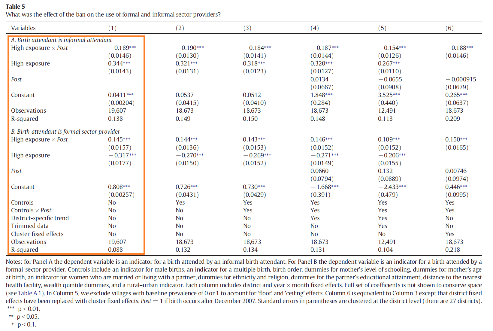
Read the notes below Table 5. See if you can modify your regression command so that your results are precisely identical to those in the paper.

Empirical Exercise

Start by creating a new do file that loads E4-GodlontonOkeke-data.dta and uses your answers to the in-class activity to generate and label the variables needed to replicate Column 1 of Table 5.

Question 1: Replicating Column 1 from Tables 5 and 6

Part (a)

Estimate a difference-in-differences specification that replicates Table 5, Panel A, Column 1. Store your results using the eststo command.

Part (b)

Now replicate Table 5, Panel B, Column 1 (the same specification with the sba dummy as the outcome variable) and store your results.

Part (c)

Recode the m3h variable to generate a dummy for having a friend or relative as the birth attendant. Use this variable to replicate Table 6, Panel A, Column 1. Store your results.

Part (d)

Now generate a variable alone that is equal to one minus the maximum of the tba, sba, and friend variables. Use this variable to replicate Table 6, Panel B, Column 1. Store your results.

Part (e)

Export your results to word (or excel if you prefer) as a nicely formatted table. Report the R-squared for each specification, and do not report coefficients on the district and time fixed effects (with esttab, use the indicate option to report which columns include fixed effects, or indicate which fixed effects are used in the table notes). Report standard errors rather than t-statistics. Make sure all variables and columns are clearly labeled, and that your labels are not cut off because they are too long.

Question 2: Assessing the Common Trends Assumption

Next, assess the validity of the common trends assumption by replicating the first two columns of Table 2 (we don’t have the outcome data needed to replicate Columns 3 and 4).

Part (a)

Drop the observations from after the ban was in place. Then, interact the time variable, which indexes the month of birth, with the high_exp variable, and label everything.

Part (b)

Replicate columns 1 and 2 from Table 2 to the best of your ability. Store your coefficient estimates.

Part (c)

Export your results to word or excel as a nicely formatted table (all of the guidance from Question 1 still applies).

Additional Activities

If you are looking for ways to expand your program evaluation skills further, extend your answer to Question 1 by including district-specific time trends, as Professor Godlonton and Dr. Okeke do in Columns 4 through 6 of Tables 5 and 6. Alternatively, you can replicate the main analysis using a continuous measure of treatment intensity: the interaction between the level of TBA use prior to the ban and the post dummy. Generate this new treatment variable using your existing meantba variable, and then estimate regressions that control for meantba and its interaction with post. How do the results from these alternative specifications compare to those reported in the paper? Finally, consider using DHS cluster fixed effects and month of birth fixed effects in the same specification. Do the DHS cluster fixed effects reduce the standard errors?

This exercise is part of the module Diff-in-Diff in Panel Data.