Empirical Exercise 5

In this exercise, we’ll be using a data set on school enrollment in 15 African countries that eliminated primary school fees between 1990 and 2015. Raw data on primary and secondary school enrollment comes from the World Bank’s World Development Indicators Database. The data set that we’ll use is posted at here. We’ll be using this data set to estimate the two-way fixed effects estimator of the impact of eliminating school fees on enrollment. Since this policy was phased in by different countries at different times, it is a useful setting for exploring the potential pitfalls of two-way fixed effects.

Getting Started

Start by creating your own R Script that downloads the data set WDI-FPE-data.csv from the web. Your code should look something like this:

fileUrl <- 'https://raw.githubusercontent.com/pjakiela/IE-in-R/gh-pages/WDI-FPE-data.csv'
E5data <- read.csv(fileUrl)

The data set contains eight variables: country, year, ccode, id, primary, secondary, fpe_year, and treatment. The variables country and year are self-explanatory. id is a unique numeric identifier for each of the 15 individual countries in the data set, and ccode is the Wold Bank’s three-letter code for each country.

The data set also contains the the variables primary and secondary which indicate gross enrollment in primary and secondary school, respectively. The gross primary enrollment ratio is 100 times the number of students enrolled in primary school divided by the number of primary-school-aged children. This number can be greater than 100 when over-age children are enrolled in primary school - which often happens when school fees are eliminated. The gross secondary enrollment ratio is defined analagously.

What is the mean of the primary variable? How does the mean in the first year included in the data set compare to the mean in the last year of the data set? Which country has the highest level of primary school enrollment?

The variable fpe_year indicates the year in which a given country made primary schooling free to all eligible children. Malawi was the first country in the data set that eliminated primary school fees (in 1994), while Namibia was the last (in 2013). The countries in the data set and the timing of school fee elimination are summarized in the table below.

ID	Country	Implementation of Free Primary Education
27	Malawi	1994
17	Ethiopia	1995
20	Ghana	1996
46	Uganda	1997
7	Cameroon	2000
44	Tanzania	2001
47	Zambia	2002
35	Rwanda	2003
23	Kenya	2003
5	Burundi	2005
31	Mozambique	2005
24	Lesotho	2006
2	Benin	2006
4	Burkina Faso	2007
32	Namibia	2013

The data set contains 15 countries, but only 13 distinct “timing groups” - since Kenya and Rwanda both eliminated primary school fees in 2003, while Benin and Lesotho both eliminated fees in 2006. The variable treatment is equal to 1 for country-years (i.e. observations in the data set) that occur after the elimination of primary school fees, and equal to 0 otherwise.

Which countries eliminated school fees in the 1990s? How many countries eliminated primary school fees after 2010?

We are going to be looking at the outcome variable primary, but this variable is missing for some country-years. How many? Add a line to your R Script that drops those observations to make your life easier (you’ll see why this matters later).

What is the mean value of primary prior to the elimination of primary school fees? How does that compare to the average level of primary enrollment after school fees are eliminated?

One-Way Fixed Effects

Before implementing two-way fixed effects to estimate the treatment effect of free primary education on gross primary enrollment, we’re going to review the mechanics of fixed effects estimation by implementing one-way fixed effects.

To do this, add a line to your do file that estimates an OLS regression of primary on treatment controlling for year fixed effects. To include fixed effects in a regression, you include the variable of interest with “i.” before it. So, for example, to include year fixed effects you would add i.year to your regression command.

Run your do file. What is the estimated coefficient on treatment when you include year fixed effects in your OLS regression?

If your code is correct, the estimated coefficient on treatment should be 10.74162, and the standard error should be 3.928681. Your regression should include 490 observations. If your results are different, go back and confirm that you have dropped the obesrvations with primary==..

There are two other ways that we can arrive at the coefficient from a fixed effects regression. As we discussed in class, one alternative to including year fixed effects is to subtract the year-level mean from both the independent variable (treatment) and the dependent variable (primary). This is a way of normalizing our values of treatment and primary across years. We can then regress our normalized (i.e. de-meaned) outcome variable on our normalized treatment variable.

To do this, we first need to use the egen command to calculate year-level means of primary and treatment. To calculate year-level means of primary, we can use the command

bysort year:  egen mean_primary = mean(primary)

Add this command to your do file, and then use similar code to calculate the year-level mean of treatment. The, write the additional code you need to generate new variables norm_primary and norm_treatment that are equal to your original variables (primary and treatment) minus the year-level means.

Now, add a line to your do file where you regress norm_primary on norm_treatment. If you have done this correctly, the estimated coefficient on norm_treatment should be the same as the coefficient on treatment in your original fixed effects regression (though the standard errors will be slightly different).

Another approach that is equivalent to fixed effects involves (first) regressing primary and treatment on your fixed effects and storing the residuals from those regressions, and then (second) regressing the residuals from your regression of primary on your fixed effects on the residuals from your regression of treatment on your fixed effects.

To implement this approach, we need to generate a variable primary_resid equal to the residuals from a regression of primary on our year fixed effects. We can do this by adding the following code to our do file:

reg primary i.year
predict primary_resid, resid

Add this code to your do file, and then write additional code that will define an analogous variable treatment_resid. Then, regress primary_resid on treatment_resid and confirm that this approach generates the same estimate of the treatment effect as either of the approaches that we used above.

You can also get the same regression coefficient by regressing primary on norm_treatment or treatment_resid - though the constant will be very different.

As we’ve discussed in class, the OLS coefficient on treatment is a linear combination of the values of the outcome variable, primary. The weights used to calculate this linear combination are proportional to our residualized treatment variable. Observations with positive values of treatment_resid get positive weight when we calculate our OLS coefficient; they are, in essence, the treatment group. Observations with negative values of treatment_resid get negavitve weight when we calculate our OLS coefficient.

What range of values of treatment_resid do you observe in our actual treatment group (observations with treatment==1)? What is the minimum value of treatment_resid in the treatment group? What is the maximum value of treatment_resid in the treatment group? What range of values of treatment_resid do you observe in our actual comparison group (observations with treatment==0)?

We can use the code below to plot the residualized values of treatment (i.e. the values of treatment_resid) by year for the treatment and comparison groups.

twoway ///
	(scatter treatment_resid year if treatment==1, mcolor(vermillion*0.8)) ///
	(scatter treatment_resid year if treatment==0, mcolor(sea*0.6)) ///
	(lpoly treatment_resid year if treatment==1, lcolor(vermillion)) ///
	(lpoly treatment_resid year if treatment==0, lcolor(sea)), ///
	legend(order(3 4) label(3 "Treatment") cols(1) label(4 "Comparison") ring(0) pos(2)) ///
	ytitle("Residualized Treatment" " ") xtitle(" " "Year")

Running this code (at the end of your existing do file) generates the following figure:

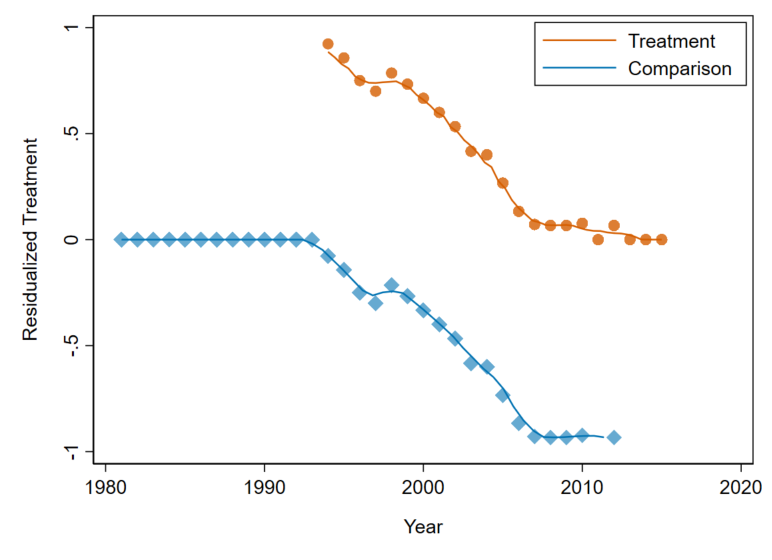
The figure illustrates a few important points:

• After including year fixed effects, years before free primary education was implemented in any of our sample countries receive zero weight in our estimation
• Years after all countries had implemented FPE also receive zero weight, as does 2011 - Namibia did not implement FPE until 2013, but date from Namibia is missing for 2011
• The country-years receiving the most positive weights are the early post-adoption years in early-adopter countries. Later adopters and later years in early-adopter countries receive much less weight
• Within the comparison group, the most weight is put on late-adopter countries in the years immediately before they adopted FPE

Two-Way Fixed Effects

Now we are ready to estimate the impact of eliminating primary school fees on gross primary enrollment using two-way fixed effects (TWFE). We want to implement the regression equation: where Y_it is the outcome variable of interest (gross primary enrollment); λ_i and γ_t are country and year fixed effects, respectively; and D_it is our treatment dummy, an indicator equal to one in country-years after the elimination of school fees (inluding the year during which school fees were eliminated).

As in the case of one-way fixed effects, there are three ways that we can arrive at the TWFE estimate of the treatment effect of free primary education:

1. By running a TWFE regression
2. By normalizing the independent and dependent variables by subtracting off the appropriate means
3. By regressing a residualized version of our outcome variable on a residualized version of our treatment variable

For this exercise, we’ll be focusing on approaches (1) and (3).

Before we work through these approaches, extend your do file so that you drop the variables that you generated in the first part of this exercise: mean_primary, mean_treatment, norm_primary, norm_treatment, primary_resid, and treatment_resid.

The TWFE Regression

Start by running a TWFE regression of primary on treatment plus year and country fixed effects. Add a line that does this at the bottom of your do file, and then run your code. What is the estimated regression coefficient on treatment? Is the coefficient statistically significant? How much does eliminated primary school fees increase gross enrollment in primary school?

Residualized Treatment

The coefficient from a two-way fixed effects regression is equal to the coefficient from a regression of your outcome on the residuals from a regression of treatment on your two-way fixed effects. To see this, regress treatment on country and year fixed effects, and the use the post-estimation predict command to generate a value equal to the residual from this regression:

reg treatment i.year i.id
predict treatment_resid, resid

Again, treatment_resid is the name of the new variable, the residual from a regression of treatment on country and year fixed effects. Regress primary on treatment_resid without any additional controls. You should see that the estimated coefficient is identical to the coefficient of interest in your original two-way fixed effects regression.

Further extend your code so that you generate a variable primary_resid in the same way that you generated treatment_resid (by regressing primary on country and year fixed effects, and then predicting the residuals). Then regress primary_resid on treatment_resid. You should once again replicate the same TWFE estimate of the treatment effect.

Is the TWFE Coefficient Biased?

In lecture, we saw that the TWFE difference-in-differences estimator does not always provide an unbiased estimate of the treatment effect that we are interested in. We can now see why. We started with a treatment dummy: treatment equals one in country-years where primary education was free, and zero in country-years when primary school fees had not yet been eliminated. So, our treatment group is country years with free primary education.

However, when we include country and year fixed effects, we convert our treatment dummy into a continuous measure of treatment intensity - specifically a measure of treatment intensity that is not explained/predicted by our country-year fixed effects.

There is an important difference between regression on a dummy variable and regression on a continuous measure of treatment intensity (as we saw in earlier modules): when we regress an outcome on (only) a treatment dummy, the estimated treated effect is a weighted average of the treatment effect on treated units (assuming there is no selection bias to worry about); but when we regress on a continous measure of treatment intensity, we are imposing a linear dose-response relationship and placing greater weight on outcomes further from the mean treatment intensity. Importantly, all observations with below mean treatment intensity are implicitly part of the comparison group.

In practical terms, we’ve seen that the TWFE coefficient puts negative weight on treated observations (i.e. country-years) where the residualized value of treatment (treatment_resid) is negative. So, the practical question is: how often does this happen among observations with treatment equal to one? Test this by summarizing the treatment_resid variable in the treatment group. What is the lowest value of treatment_resid that you observe in the treatment group? How many treated observations are there, and how many of them have values of treatment_resid that are less than zero?

You can use the following code to compare the distributions of the the treatment_resid variable in the treatment and comparison groups:

tw ///
 (histogram treatment_resid if treatment==0, frac bcolor(vermillion%40)) ///
 (histogram treatment_resid if treatment==1, frac bcolor(sea%60)), ///
 xtitle(" " "Residualized Treatment") ///
 legend(label(1 "Comparison") label(2 "Treatment") col(1) ring(0) pos(11)) ///
 plotregion(margin(vsmall))

We can see that the residualized value of treatment is negative for quite a few country-years in the treatment group (when primary education was free). We know from lecture that this occurs because the value of treatment predicted from our regression of treatment on country and year fixed effects is greater than one. Hence, country-year observations receiving negative weight in our TWFE regression are those in countries where the mean level of treatment is high (early adopters of free primary education) in years when the average level of treatment is high (later years, after most countries implemented free primary education).

To confirm that this is the case, generate a variable negweight equal to one if a country-year has treatment==1 and treatment_resid<0.
Tabulate the country variable among observations where this negweight variable is equal to one. Which country has the highest number of treated years receiving negative weight in our two-way fixed effects estimation? When did that country implement free primary education?

Truncating the Data Set to Eliminate Negative Weights

Negative weights arise because the predicted value of treatment is greater than one for some treated observations. This occurs for country-years where both the country-level-mean and the year-level-mean of the treatment variable are high - i.e. in early-adopter countries observed in later years of the panel (by which time most countries are treated). One way to eliminate negative weights, so that we only place positive weight on treated country-years, is to truncate the data set before late-adopter countries are treated. If treatment effects are homogenous, this should not change your estimated treatment effect too much (though your data set will be smaller, so your standard errors will probably be larger).

To see that this is the case, extend your do file so that you drop observations after 2005. Re-run the two-way fixed effects estimation in this restricted sample. What is the estimated coefficient on treatment? How different is it from your initial estimate?

Now regress treatment on your country and year fixed effects, and then predict the residuals (you will either need to drop treatment_resid first or give your new variable a name other than treatment_resid). These are the relative weights used in your two-way fixed effects estimation of the impact of treatment on primary school enrollment. Summarize the regression weights for observations in the treatment group. How many are negative? What is the lowest weight placed on a country-year observation where treatment==1?

Wrapping Up

Before you submit your do file on grade scope, make sure it does the following:

1. Loads the data set form github
2. Drops observations for which the primary variable is missing
3. Regresses primary on treatment controlling for year fixed effects
4. Uses the egen command to generate year-level means of treatment and primary
5. Generates normalized variables norm_primary and norm_treatment constructed by subtracting off the year-level means of each variable
6. Regresses norm_primary on norm_treatment to obtain the same one-way fixed effects coefficient that you got in Question 3
7. Generates residualized variables treatment_resid and primary_resid from regressions of each variable on year fixed effects.
8. Regresses primary_resid on treatment_resid to obtain the same coefficient estimate as in Question 3
9. Drops the variables mean_primary, mean_treatment, norm_primary, norm_treatment, primary_resid, and treatment_resid (to begin your analysis of two-way fied effects)
10. Implements a two-way fixed effects regression of primary on treatment including year and country fixed effects
11. Generates new variables treatment_resid and primary_resid from regressions on year and country fixed effects
12. Regresses primary on treatment_resid and primary_resid on treatment_resid to show that both approaches generate the same two-way fixed effects estimate of the treatment effect
13. Generate a variable negweight equal to one if a country-year has treatment==1 and treatment_resid<0, and tabulates the country variable among observations where this negweight variable is equal to one to identify observations receiving ngeative weight in our analysis
14. Estimates two-way fixed effects estimation in a restricted sample that drops years after 2005
15. Determines what fraction of treated observations in the restricted sample are receiving negative weight in our two-way fixed effects estimation

More Fun with Stata

We can also calculate the difference-in-differences estimator “by hand” from the observed values of the primary and treatment_resid variables. We know that when we run a univariate regression in a data set containing a totla of n observations, the OLS coefficient can be written as:

In this case, our right-hand side variable (X in the equation above) is the residualized treatment variable treatment_resid. It has a mean of zero (the residuals from a regression are mean-zero by construction) - so we don’t need to worry about the “X-bar” terms. This means that we can calculate the two-way fixed effects difference-in-differences estimator using the following code:

gen yxtresid = primary*treatment_resid
egen sumyxtresid = sum(yxtresid)
gen tresid2 = treatment_resid^2
egen sumtresid2 = sum(tresid2)
gen twfecoef = sumyxtresid/sumtresid2
sum twfecoef
display r(mean)

In the first line, we calculate a variable that is the value of the outcome variable multiplied by the associated residual from a regression of treatment on country and year fixed effects. We then use the egen command to sum these terms across all observations. In the next two lines, we sum up the observation-level values of the square of our residualized treatment variable. The last three lines use these two sums - which appear in the algebra above - to caluculate the TWFE estimator of the treatment effect by hand (in some sense).

If you have done this correctly, you will see that our original two-way fixed effects coefficient, the coefficient from our regression of primary on treatment_resid, and the mean of our new variable twfecoef are all identical (though the associated standard errors are different). Thus, we’ve shown that the two-way fixed effects coefficient is a weighted sum of the values of the outcome variable (like any coefficient from a univariate OLS regression).