Empirical Exercise 11 in Python

In this exercise, we’ll learn how to determine the appropriate sample size for cluster-randomized trials. Researchers often assign treatment at the cluster level (e.g. at the school, community, or market level) when we are worried about potential spillovers across individuals within a cluster. However, if outcomes within a cluster are correlated (as they usually are), we need to modify our approach to calculating statistical power and sample size.

Getting Started

Create a program that contains the following code:

# preliminaries -----------------------------------
import numpy as np
import pandas as pd
import statsmodels.formula.api as smf

# setup -------------------------------------------
np.random.seed(24601)
numclusters = 100
obspercluster = 1
effect = 0
loopmax = 1000

## empty vector to store results
pvals = np.full(loopmax, np.nan)

# create clustered data ---------------------------

for i in range(1, loopmax + 1): 
    print("Loop iteration: ", i)
    j = i - 1
    data = pd.DataFrame({'clustid': np.arange(1, numclusters+1, 1), 
                         'clusteffect': np.random.randn(numclusters)})
    data['treatment'] = np.where(data['clustid'] >= numclusters/2, 1, 0)
    data = data.loc[np.repeat(data.index.values, obspercluster)].reset_index(drop=True)
    data['y'] = data['clusteffect'] + effect*data['treatment'] + np.random.randn(numclusters*obspercluster)
    ols = smf.ols('y ~ treatment', data = data).fit()
    pvals[j] = ols.pvalues.iloc[0]

significant = np.where(pvals < 0.05, 1, 0)
print(significant.mean())

The code generates (i.e. simulates) a data set that is clustered: observations are grouped into clusters, and outcomes (even in the absence of treatment) are correlated within each cluster. So, for example, this could be a data set of student test scores where the individual unit of observation is the student and the cluster is the classroom; students within a classroom are in the same grade and the same school, have the same teacher, and talk to each other - so we might expect their test scores to be correlated.

The numclusters parameter indicates the number of clusters in the similuated data set, and the obspercluster parameter indicates the number of observations per cluster. As you can see, the current values of those parameters create a data set with only one observation per cluster (so this is a clustered data set in name only at this point, though you will fix that shortly).

The line

pvals = np.full(loopmax, np.nan)

allows you to create an empty vector where you can store results. np.full() defines a repeating vector or matrix: for example np.full((10, 8), 1) would define a matrix of ones (the second argument) with 10 rows and 8 columns. Here we define an empty vector with loopmax rows and one column. We can use this to record the p-values that we calculate in our simulations.

In-Class Activity

Question 1

Look carefully at the code. Make sure you understand what is happening in every line (and if you do not, come ask me to explain anything that is confusing). What is the mean of the treatment variable (in each iteration of the loop)? You should be able to figure this out without running the code.

Question 2

Looking at the current values of the parameters defined in the setup section, would you say that the null hypothesis is true or false?

Question 3

When you run the code and it tabulates the significant variable at the end, what is the expected number of times that you will reject the null hypothesis?

Question 4

Now run the code. How many times do you actually reject the null hypothesis?

Question 5

Change the number of iterations (the number of times the loop runs) to 1,000, and then run the code again. How many times do you reject the null hypothesis now? Was this what you expected?

Question 6

Recall the formula for the minimum detectable effect from last week:

mde

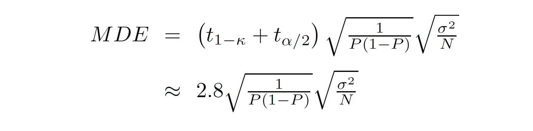
The square root terms (together) are the expected value of the standard error of the estimated treatment effect. The P in the equation is the proportion of the sample that is treated, which in this case is… the answer to Question 1; and the sample size is the number of clusters times the number of observations per cluster. To calculate the expected standard error, you still need the variance of the outcome variable, σ².

Notice that y is the sum of a cluster-specific error term, which is normally distributed with mean zero and variance one, and an observation-specific error term, which is also a standard normal - plus a treatment effect which is zero at present, but is in any case not stochastic. So, y is a random variable that is the sum of two independent standard normals. We know that the variance of two independent random variables is the sum of their variances. Given this, what is the variance of y? (I am asking for the expected or population variance, not the sample variance that you would get by running the code.)

Question 7

Now use the MDE formula to calculate the expected standard error in the regression of y on treatment. What is it?

Question 8

Now modify the code so that you also save the standard error from the regression of y on treatment. What is the average standard error across your 1,000 simulations?

Question 9

You can multiply the expected standard error by 2.8 to calculate the MDE given a test size of 0.05 and a power of 0.8. This tells us that the MDE is approximately 0.25. Change the parameter effect to 0.25 and run your code again. In how many of your 1,000 simulations do you reject the null hypothesis?

Question 10

Now consider a case where treatment is assigned at the cluster level, and there are multiple observations per cluster. Change numclusters to 50 and obspercluster to 20. The code

data = data.loc[np.repeat(data.index.values, obspercluster)].reset_index(drop=True)

will make obspercluster identical copies of all of your observations, so that you will have 1000 observations in total. Now, set effect to 0 again, so that the null hypothesis (that treatment has no effect) is correct. Run your code. How many times (out of 1,000) do you reject the null?

Question 11

When treatment is assigned at the cluster level and outcomes are correlated within clusters, hypothesis tests are incorrectly sized unless we use the cluster option at the end of our regression. Run your code again after replacing the regression specification with:

ols = smf.ols('y ~ treatment', data = data).fit(    
    cov_type='cluster', 
    cov_kwds={'groups': data['clustid']})

How many times to you reject the null hypothesis now?

Empirical Exercise

In the remainder of this exercise, we will extend the simulation program that we used in the in-class activity. To get started, create a new program containing the same simulation program that we used above (with 50 clusters, 20 observations per cluster, and a treatment effect of 0). Extend your code as you answer the following questions.

Question 1

As we’ve seen, when treatment is assigned at the cluster elvel, our hypothesis tests are only correctly sized when we cluster our standard errors. How do we account for this in calculating statistical power or required sample size? For cluster-randomized trials, we use a slightly different equation for the MDE:

MDE-clusters

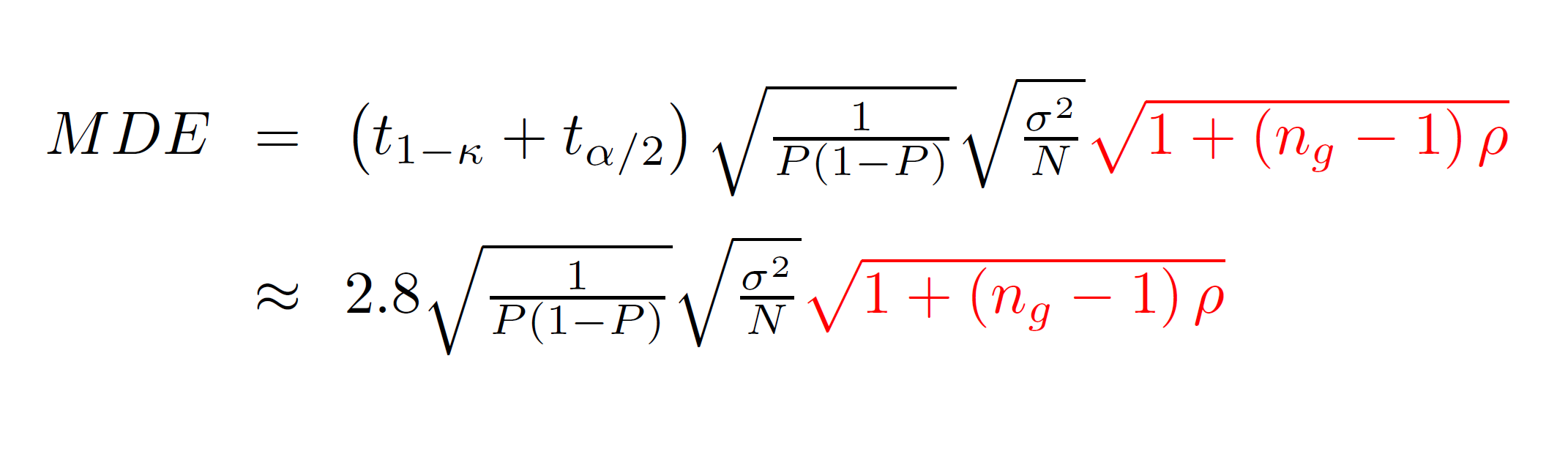
The term in red did not appear in the version of the MDE equation that we used before. That term is referred to as the Moulton factor. It is always weakly greater than one, indicating that cluster-randomized trials have less power than individually-randomized trials. The Moulton factor depends on two terms: n_g is the average number of observations per group and ρ is the intra-class correlation, a measure of how correlated outcomes are within clusters. Development economists usually assume levels of intra-class correlation between 0 and perhaps 0.2 and 0.3. Student test scores among students with the same teacher tend to be very highly correlated; other outcomes (for example, the incomes of people in the same village) are usually be less highly correlated.

You can use the code below to estimate the degree of intraclass correlation, ρ, and store your estimates (in an empty vector rho that you create). Add this code to your loop after you store the results from the main regression of y on treatment:

rho_model = smf.mixedlm('y ~ 1', data, groups=data['clustid']).fit()
var_group = rho_model.cov_re.iloc[0, 0]
var_resid = rho_model.scale
rho[j] = var_group / (var_group + var_resid)

What is the mean level of intra-class correlation across your 1,000 simulations?

Question 2

Given this level of intra-class correlation, what does the MDE formulate indicate is the MDE in this data set?

Question 3

Change the value of effect to be equal to the MDE that you calculated in Question 2, and then run your code. How many times (out of 1,000) do you reject the null hypothesis?

Question 4

With an individually-randomized sample of N=1000, we were powered to detect an effect of about 0.25 (given the variance of the outcome was 2). With an intra-class correlation of 0.4956562 and a resulting Moulton factor of 3.22761, how large of a sample would we need to obtain that MDE (of 0.25)? Use the MDE formula to answer this question.

Question 5

Confirm that, with the sample size you have calculated, you are powered to detect an MDE of 0.25 using your simulation code.

Question 6

An intra-class correlation of about 0.5 is very high. Even among students within the same classroom in the same school, the intra-class correlation is often closer to 0.1 or 0.2.

Part (a)

How large of a sample would you need to be powered to detect an impact of 0.25 if the intra-class correlation were 0.2?

Part (b)

How large of a sample would you need to be powered to detect an impact of 0.25 if the intra-class correlation were 0.05?

Extensions

How would you calculate the required sample size if you expected 10 percent attrition between baseline and endline in both the treatment group and the control group?
How would you calculate the required sample size if you only expected 50 percent take-up among individuals assigned to treatment?

This exercise is part of the module Clustering.