Empirical Exercise 11, Part C

In this exercise, we’ll learn how to determine the appropriate sample size for cluster-randomized trials. As discussed in Running Randomized Evaluations, researchers often assign treatment at the cluster level (e.g. at the school, community, or market level) when we are worried about potential spillovers across individuals within a cluster. However, if outcomes within a cluster are correlated (as they usually are), we need to modify our approach to calculating statistical power and sample size.

Getting Started

The do file below generates (i.e. simulates) a data set that is clustered: observations are grouped into clusters, and outcomes (even in the absence of treatment) are correlated within each cluster. So, for example, this could be a data set of student test scores where the individual unit of observation is the student and the cluster is the classroom; students within a classroom are in the same grade and the same school, have the same teacher, and talk to each other - so we might expect their scores to be correlated.

The local macro numclusters indicates the number of clusters in the similuated data set, and the local macro obspercluster indicates the number of observations per cluster. As you can see, the current values of those macros create a data set with only one observation per cluster (so this is a clustered data set in name only at this point - though you will fix that shortly).

clear all
set seed 24601

local numclusters = 1000
local obspercluster = 1
local effect = 0

// create an empty matrix to save results

local loopmax=100
matrix pval=J(`loopmax',1,.)

// create data sets w/ clusters

forvalues i  =1/`loopmax' {
    display "Loop iteration `i'"
	set obs `numclusters'
	gen clustid = _n
	gen treatment=cond(_n>`numclusters'/2,1,0)
	gen clusteffect = rnormal()
	gen y = clusteffect + `effect'*treatment + rnormal()
	reg y treatment
	mat V = r(table)
	matrix pval[`i',1]=V[4,1]
	drop clustid treatment clusteffect y
}

svmat pval
summarize
gen significant = pval<0.05
tab significant

The line

matrix pval=J(`loopmax',1,.)

is new. The matrix command allows you to create (unsuprisingly) a matrix where you can store results. Using the matrix command with the function J defines a repeating matrix: for example matrix X = J(10,8,1) would define a matrix one ones with 10 rows and 8 columns. Here we define an empty matrix with loopmax rows and one column (so, really, it is a vector). We can use this to record the p-values that we calculate in our simulations.

We use the matrix command again inside the loop. The command mat V = r(table) saves the results of a regression in the matrix V. For example, suppose you ran the command reg y x1 x2 and saw the Stata output below.

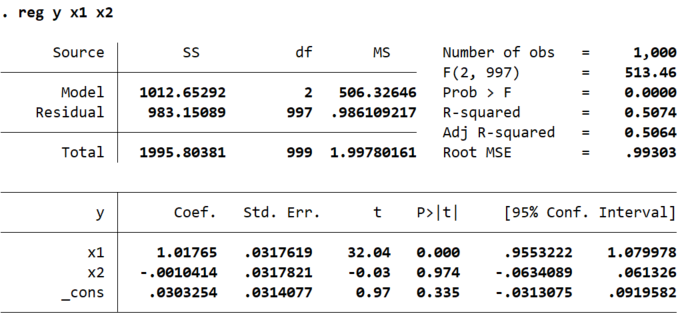
If you ran the command mat V = r(table) and then used the command mat list V to display the matrix, you’d see this:

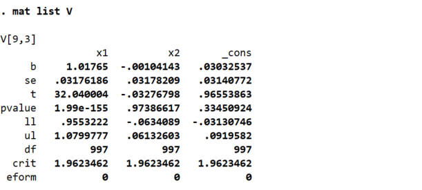
You can see that Stata has now created a 9x3 matrix that contains all the estimated coefficients, standard errors, t-statistics, p-values, etc. from the regression. The columns of the matrix represent the independent variables in the regression, in the order that you entered them. The last column reports the estimated constant term, its standard error, etc.

In our loop, we save our regression results in the matrix V and then immediately save the p-value associated with the treatment variable (the only independent variable in our regression) as one term in the pval vector that we defined prior to running the loop. This means that, once our loop has run through all 100 iterations, we’ll have a vector containing all 100 resulting p-values, which we can then save as a variable using the svmat command.

Empirical Exercise

Question 1

Look carefully at the program. Make sure you understand what is happening in every line (and if you do not, come ask me to explain anything that is confusing!). What is the mean of the treatment variable (in each iteration of the loop)? You should be able to figure this out without running the code.

Question 2

Looking at the current values of the local macros, would you say that the null hypothesis is true or false?

Question 3

When you run the code and it tabulates the significant variable at the end, what is the expected number of times that you will reject the null hypothesis?

Question 4

Now run the code. How many times do you actually reject the null hypothesis?

Question 5

Change the number of iterations (the number of times the loop runs) to 1,000, and then run the code again. How many times do you reject the null hypothesis now?

Question 6

Recall the formula for the minimum detectable effect from last week:

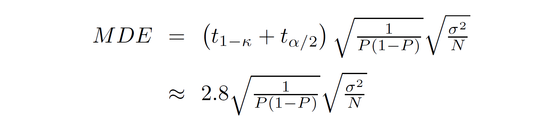
The square root terms (together) are the expected value of the standard error of the estimated treatment effect. The P in the equation is the proportion of the sample that is treated, which in this case is… the answer to Question 1; and the sample size is the number of clusters times the number of observations per cluster. To calculate the expected standard error, you still need the variance of the outcome variable, σ².

Notice that y is the sum of a cluster-specific error term, which is normally distributed with mean zero and variance one (because the rnormal() command takes draws from a standard normal random variable), and an observation-specific error term, which is also a standard normal - plus a treatment effect which is zero at present, but is in any case not stochastic. So, y is a random variable that is the sum of two independent standard normals. We know that the variance of two independent random variables is the sum of their variances. Given this, what is the variance of y? (I am asking for the expected or population variance, not the sample variance that you would get by running the code.)

Question 7

Now use the MDE formula to calculate the expected standard error in the regression of y on treatment. What is it?

Question 8

Now modify the program so that you also save the standard error from the regression of y on treatment. (You will need to create a new blank matrix to store the estimated standard errors in.) What is the average standard error across your 1,000 simulations?

By the way, if you are frustrated that your code is taking too long to run, you can insert the word quietly before your reg, gen, and set obs commands to speed things up.

Question 9

Now you can multiply the expected standard error by 2.8 to calculate the minimum detectable effect given a test size of 0.05 and a power of 0.8. This tells us that the MDE is approximately 0.25. Change the local macro effect to 0.25 and run your code again. In how many of your 1,000 simulations do you reject the null hypothesis?

Question 10

Check your answer by using the sampsi command to calculate the number of observations that you’d need to detect a difference in means between a mean of 0 in one group and a mean of 0.25 in another group given a power of 0.8 and a standard deviation of 1.4142136. What would be the required sample size (n1+n2)?

Question 11

Now consider a case where treatment is assigned at the cluster level, and there are multiple observations per cluster. Change the local macro numclusters to 50 and the local macro obspercluster to 20. Then, insert the command

quietly expand `obspercluster'

between the gen clusteffect... and gen y=... commands. The expand command will make obspercluster identical copies of all of your observations (within your data set), so that you will have 1000 observations in total. Now, set effect to 0 again, so that the null hypothesis (that treatment has no effect) is correct. Run your code. How many times (out of 1,000) do you reject the null?

Question 12

When treatment is assigned at the cluster level and outcomes are correlated within clusters, hypothesis tests are incorrectly sized unless we use the cluster option at the end of our regression. Run your code again, but add , cluster(clustid) to the end of your regression. How many times to you reject the null hypothesis now?

Question 13

As we’ve seen, when treatment is assigned at the cluster elvel, our hypothesis tests are only correctly sized when we cluster our standard errors. How do we account for this in calculating statistical power or required sample size? For cluster-randomized trials, we use a slightly different equation for the MDE:

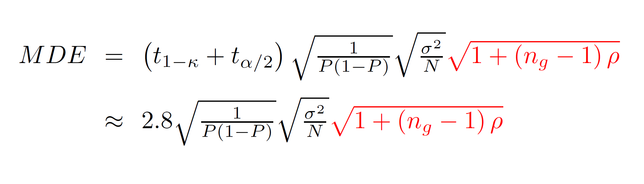
The term in red did not appear in our earlier equation. That term is referred to as the Moulton factor. It is always greater than one, indicating that cluster-randomized trials have less power than individually-randomized trials. The Moulton factor depends on two terms: n_g is the average number of observations per group and ρ is the intra-class correlation, a measure of how correlated outcomes are within clusters. In development, we typically think about levels of intra-class correlation between 0 and perhaps 0.2 and 0.3. Student test scores among students with the same teacher tend to be very highly correlated; other outcomes (for example, the incomes of people in the same village) might be less highly correlated.

We can use the stata command loneway to estimate the degree of intraclass correlation, ρ. Modify your code so that you create an empty matrix rho (just like the empty matrix pval) where you can store your estimates of the intraclass correlation, and then add this code to your loop immediately before the drop command:

loneway y clustid
matrix rho[`i',1]=r(rho)

Then add an svmat rho command near the end of your do file. What is the mean level of intra-class correlation across your 1,000 simulations?

Question 14

Given this, what is the MDE?

Question 15

Change the value of the local macro effect to be equal to the MDE that you calculated in Question 14, and then run your code. How many times (out of 1,000) do you reject the null hypothesis?

Congratulations!

You finished all the empirical exercises in ECON 379! Hurray! And now you know how to calculate the required sample size for an individually-randomized or a cluster-randomized study. The level of intra-class correlation in our simulations was extremely high - much higher than we’d typically observe in an outcome variable of interest. However, as you saw above, cluster-randomized trials often require substantially larger samples than individually-randomized studies (or, equivalently, they are only able to detect substantially larger treatment effects).