Empirical Exercise 11, Part 2

This is the second of two exercises on power calculations in indiviudal-level randomizations. In this exercise, we’ll review the concepts of size and power in hypothesis testing, and learn how to calculate the minimum detectable effect as a function of sample size (or the required sample size as a function of the minimum detectable effect).

wahlberg

What Is Power?

Every time we test a hypothesis, we make a decision about whether or not to reject a null hypothesis in favor of an alternative. In impact evaluation, the null hypothesis is usually “This intervention has no impact.” When we reject that null hypothesis, we are saying “We think this intervention has an impact” - but we could always be wrong. It could be that the stars (or, more precisely, the error terms in our model) align to make it look like outcomes are different in the treatment and the comparison group, even when an intervention actually did nothing. It is also possible for the stars to align the other way, making it look like a treatment has no (statistically significant) effect when that is not correct.

In the last exercise, we learned that the size of a hypothesis test is the probability of a Type I error (rejecting a null hypothesis that is actually true - i.e. “finding” an effect that isn’t actually there). Ever since Fisher, it has been standard to use a test size of 0.05, which means that we expect to reject a true null hypothesis about 5 percent of the time.

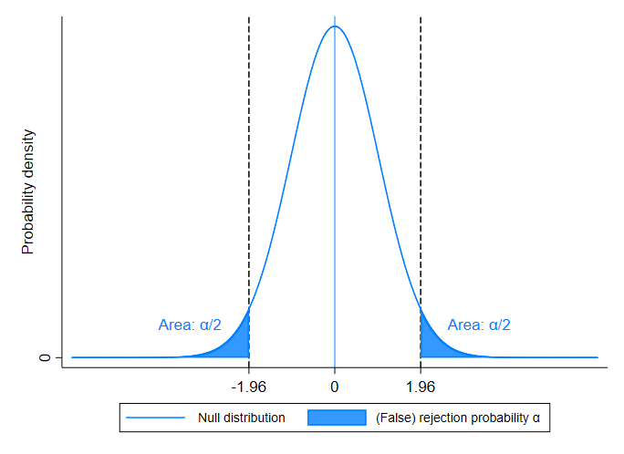
When we estimate a difference in means, we’re usually thinking about a test statistic that has a normal (or t) distribution. Under the null hypothesis of no treatment effect, the estimated impact will be distributed around a mean of zero. (In other words, if we did our experiment thousands of times, we’d expect the estimated impact to be zero on average - but it would sometimes be positive and sometimes be negative. The estimated impact would usually be small relative to the standard error - implying a relatively low t-statistic - but sometimes it would be fairly large, and would appear statistically significant.) When expressed in terms of a t-statistic, we know that the absoluted value will be greater than 1.96 about 5 percent of the time (this is why, when we see a t-statistic larger than 1.96 in absolute value, we say that the effect is statistically significant at the 95 percent confidence level).

Consider a concrete example. Suppose that you randomly assign treatment in a sample of 1,000 people so that 500 are in the treatment group and 500 are in the control group. There are a lot of different possible random assignments (i.e. a lot of different sets of 500 out 1,000 people that you could choose to include in the treatment group). You regress some outcome variable - let’s say adult height - on your treatment dummy in each of these samples - without actually implementing an intervention of any kind. So, the null hypothesis is true: the treatment effect is zero because we didn’t actually implement any treatment. Nevertheless, adult height will sometimes be significantly higher in the treatment group, just by chance. When we say that a result is statistically significant at the 95 percent level, we are choosing a threshold for significance such that adult height will be statistically significant in 5 percent of all the regressions we run when the null hypothesis (that there is no treatment effect) is correct.

Why don’t we use a smaller test, so that we have a lower probability of a Type I error? The problem is that when we reduce the size of the test, we also reduce the power (the probability of rejecting a false null hypothesis, ie the chance that we notice an impact that is actually there). Using a smaller test size means that we need to see a bigger difference in means between the treatment and comparison groups before we deem an impact “statistically significant.” When we do this, it makes it less likely that we will reject a true null hypothesis by mistake, but it also raises the bar on how large a treatment effect needs to be (in expectation) before we declare it significant.

The power of a test is the probability of rejecting a false null hypothesis, i.e. the chance of “finding” an effect that is actually there. The power of a test is one minus the probability of a Type II error (failing to reject a false null hypothesis). When we do a power calculation, we are trying to figure out the likelihood that we will be able to detect an effect of a given size with the sample we have. In other words, we’re asking “If the true effect is this big, what is the probability that we end up with an estimated t-statistic larger (in magnitude) than 1.96?” In this context, when we talk about an effect “of a given size” we are measuring the size of the treatment effect in units equivalent to the standard error of the test statistic under the null (because we want to know the probability that we’ll get a t-statistic of at least 1.96 in absolute value).

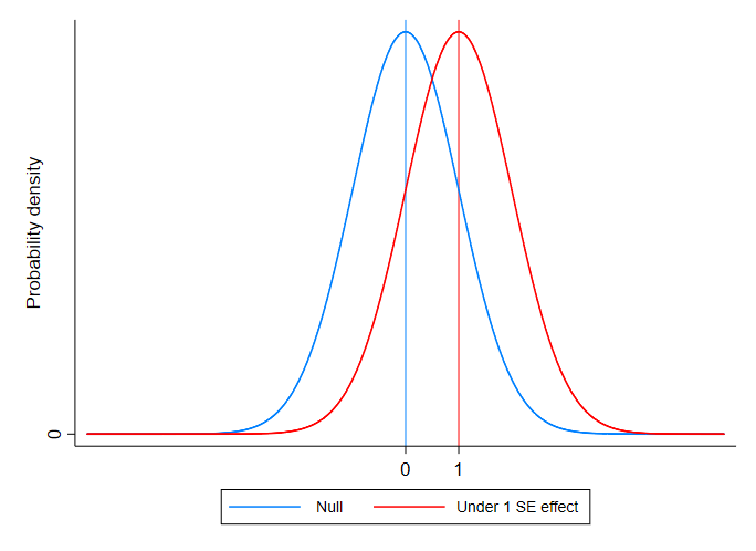
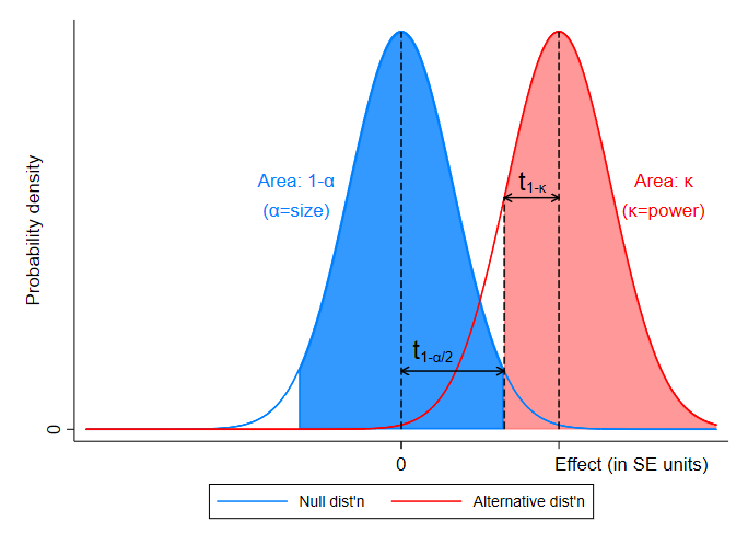
Suppose we thought that our treatment were going to increase the mean of the outcome variable by an amount equivalent to one standard error of the estimated treatment effect. If that were the case, then our test statistic would have the distribution depicted in red in the figure below. (The blue curve represents the distribution of the statistic under the null.) As you can see, the two distributions are actually pretty similar: a treatment effect equivalent to one standard error means that range of t-statistics we’d expect is not very different from what we’d expect under the null.

t1a

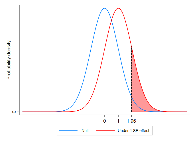
If a program increases outcomes by one standard error, the probability that we get a test-statistic large enough to reject the null (the power of our test) is actually pretty low, as you can see in the figure below. The power is the shaded pink area: the proportion of the red pdf of the test statistic (under the alternative hypothesis) that falls to the right of the critical value of the distribution of the test statistic under the null.

t1c

If we instead consider a case where the treatment effect is three times as large as the standard error the test statistic under the null, we can see that the red and blue pdfs are now quite different - and the probability of detecting a treatment effect is quite large.

t3c

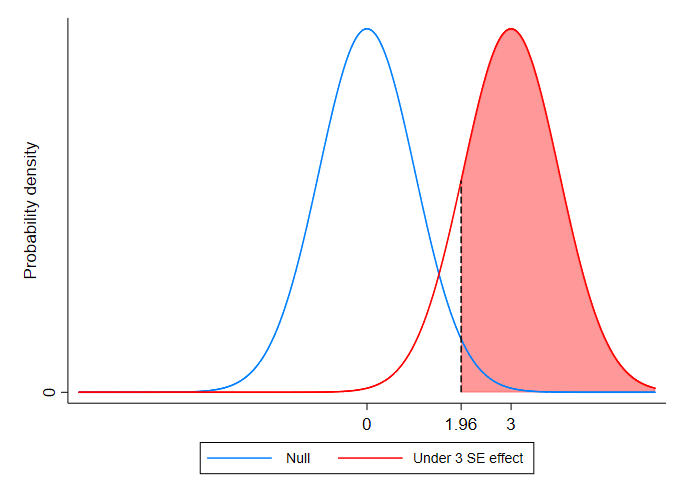
We usually look for a power of at least 0.8, by which we mean that we want to probability of detecting an effect (if there is one) to be at least 0.8. In practice that means that we want 80 percent of the area under the red curve to be to the right of the critical value (of 1.96) of the distribution of t-statistics under the null (the blue curve). You can see an example of this in the figure below.

tPC

In practice, we can frame the question of power in two ways:

Given a sample size, how large of an impact can I detect (if I require a power of at least 0.8)?
Given an effect size (expressed in terms of standard errors), how large of a sample do I need to ensure that I have a power of at least 0.8?

Which approach makes sense will depend on the context: if our sample size is fixed (for example, if you are doing an intervention in with a pre-existing sample of survey respondents), it makes sense to ask how large of an impact you can detect (and whether an impact of that magnitude is plausible given the nature of your outcome variable); if you are starting from scratch, it might make more sense to ask what size of an impact you should expect (based on, for example, evidence from other studies) and calculate the sample size you need as a result.

Empirical Exercise

In this exercise, we’ll be using data from two experiments that we’ve already studied. The first of these is the impact evaluation of malaria treatment that we studied in the first week of class. The data set E1-CohenEtAl-data.dta contains (some of the) data from Price Subsidies, Diagnostic Tests, and Targeting of Malaria Treatment: Evidence from a Randomized Controlled Trial by Jessica Cohen, Pascaline Dupas, and Simone Schaner, a paper that appeared in the American Economic Review in 2015. The authors examine behavioral responses to various discounts (“subsidies”) for malaria treatment, called “artemisinin combination therapy” or “ACT.”
The J-PAL summary of the experiment and the findings is here.

Create a do file that uses the following code to download the data.

clear all 
set scheme s1mono 
set more off
set seed 12345
version 16.1

cd "C:\Users\pj\Dropbox\econ379-2021\exercises\E11-power"

** load data 
webuse set https://pjakiela.github.io/ECON379/exercises/E1-intro/
webuse E1-CohenEtAl-data.dta

Question 1

Your are designing an intervention intended to increase knowledge about malaria transmission. Your main outcome variable of interest is b_knowledge_correct. Summarize this variable using the sum command with the detail option. What is the estimated standard deviation of b_knowledge_correct?

Question 2

What is the estimated variance of b_knowledge_correct?

Question 3

Using the formula for the minimum detectable effect, calculate the MDE given your sample size if you assume equally-sized treatment and comparison groups (so P in the formula = 0.5). What is the MDE?

Question 4

Now use the sampsi command to calculate the sample size you would need to detect an MDE equal to your answer to Question 3, given the standard deviation of the outcome variable. What sample size does sampsi indicate that you need?

Question 5

The treatment dummy in the original study is act_any. Based on this variable, what is the ratio of treated obesrvations to control observations?

Question 6

Use the formula to calculate the MDE in the study (if you used the same outcome variable as above, b_knowledge_correct) given the actual ratio of treatment to control observations. What is the MDE?

Question 7

Now use the sampsi command to check your answer. The ratio() option allows you to indicate a ratio of treatment:comparison observations that differs from one (note that this is not the same as the proportion of observations that are treated). What is the required sample size that you would need to detect an impact as large as your answer to Question 6?

Question 8

One way to increase power is to include controls that explain the observed variation in the outcome variable. When you plan to include controls, the standard deviation used in the MDE calculuation is the standard deviation of the the residuals after regressing the outcome on the controls. Replace the missing values of the variables b_acres with zeroes. Then, regress b_knowledge_correct on b_h_edu, b_hh_size, b_acres, and b_dist_km. Use the post-estimation command predict to predict the residuals, generating the new variable yresid. Then summarize yresid. What is the standard deviation of the outcome variable after regressing on the controls?

Question 9

Using the standard deviation of the residualized outcome variable, calculate the MDE (using the assumptions about the ratio of treatment and control observations that you used in Question 6). What is the MDE?

Question 10

What is the mean of the outcome variable, b_knowledge_correct?

Question 11

Express the MDE as a perecentage of the outcome variable of interest: how large of a (percent) change in b_knowledge_correct would we need to anticipate if we wanted to have power of 0.8 to detect it?

Question 12

Now we will consider a completely different data set: the data on access to microfinance that we used in Empirical Exercise 8. The data comes from the paper The Miracle of Microfinance? Evidence from a Randomized Evaluation by Abhijit Banerjee, Esther Duflo, Rachel Glennerster, and Cynthia Kinnan. The paper reports the results of one of the first randomized evaluations of a microcredit intervention. The authors worked with an Indian MFI (microfinance institution) called Spandana that was expanding into the city of Hyderabad. Spandana identified 104 neighborhoods where it would be willing to open branches. They couldn’t open branches in all the neighborhoods simultaneously, so they worked with the researchers to assign half of them to a treatment group where branches would be opened immediately. Spandana held off on opening branches in the control neighborhoods until after the study.

Use the code below to read the data into Stata and drop the observations where our outcome variable of interest, bizprofit_1, is missing:

clear
webuse set https://pjakiela.github.io/ECON379/exercises/E8-TOT/
webuse E8-BanerjeeEtAl-data.dta
drop if bizprofit_1==.

Look at a histogram of the bizprofit_1 variable. What do you notice about its distribution? Now use the sum command with the detail option. What is the mean of bizprofit_1?

Question 13

What is the standard deviation of bizprofit_1?

Question 14

Given the size of this data set and the standard deviation of bizprofit_1, what is the MDE if you wanted to have power of 0.8 (assuming treatment and comparison groups of equal size)?

Question 15

How does this MDE compare to the mean of the outcome variable? How large of a percent change in the outcome would you need to anticipate if you wanted to have power of at least 0.8?