Empirical Exercise 11

This is the first of two exercises on power calculations. In this exercise, we’ll review the concepts of size and power in hypothesis testing, and learn how to calculate the minimum detectable effect as a function of sample size (or the required sample size as a function of the minimum detectable effect).

What Is a Research Design?

Every research design involves:

A null hypothesis and either one or several alternative hypotheses
A statistic related to our hypotheses that we can calculate from observations of an outcome variable
A rule that maps possible values of the statistic into decisions about whether to reject the null hypothesis

Example 1. We want to test the null hypothesis that a coin is “fair” (equally likely to land on heads or tails). Our statistic is the percentage of the time the coin lands on heads in 2 tosses. What are some possible rules we might use to tell us when to reject the null hypothesis?

Example 2. We want to test the hypothesis that economics majors know more about Stata than English majors. We have data measuring performance on a Stata proficiency test for four students: two English majors and two econ majors. How can we use the data to decide whether to reject the null hypothesis that econ majors and English majors are equally proficienct with Stata?

Whenever we specify a rule about when to reject the null hypothesis, we have to worry about the possibility of getting it wrong. One possibility is that the null hypothesis is correct, but (based on our rule) we reject it. This is called a Type I error or a false positive. We also have to worry about the possibility that the null hypothesis is wrong, but (based on our rule) we fail to reject it. This is called a Type II error or, less commonly, a false zero. It is not usually possible to reduce the probabilities of both Type I and Type II errors to zero; reducing the probability of a Type I error usually involves increasing the probability of a Type II error.

We refer to the probability of a Type I error as the size of a test. The convention (dating back to Ronald Fisher) is to use a test of size 0.05. This means that we reject the null hypothesis whenever our statistic has a p-value of 0.05 or less (meaning that a statistic at least that large would occur less that five percent of the time under the null).

In the coin flip example above, the only rule that guarantees that probability of a Type I error is below 0.05 is the rule don’t ever reject the null hypothesis (which is not very helpful in terms of statistical practice). If, for example, we reject the null when we oberve either two heads or two tails, we would reject the null with probability 0.5 even if the null hypothesis was correct. In other words, we would have a test of size 0.5 instead of 0.05.

Empirical Exercise, Part 1

The Stata code below can be used to simulate our second example. It generates a sample of size N=4 comprising two treated observations (economics majors) and two untreated observations (English majors). The outcome variable y is a student’s normalized score on a test of Stata proficiency; the test is scaled so that the mean score is zero and the scores have a standard deviation of one. In our simulation, we assume scores are drawn from a standard normal distribution.

The loop does the following: first, it randomly generates draws from a standard normal to simulate test scores in a sample of N=4 under the null hypothesis of no treatment effect (of being an economics major); then it tests whether Stata proficiency is higher among the economics majors (treatment) than the English majors (control) using a particular rule for determining whether to reject the null hypothesis. It does this 100 times.

clear all
set seed 314159
set obs 100
gen id= _n

local sample = 4
gen treatment = 0 if id<=`sample'
replace treatment = 1 if id<=`sample'/2

gen reject = 0

forvalues i = 1/100 {
   gen y = rnormal() if treatment!=.
   sum y if treatment==1
   local t_min = r(min)
   sum y if treatment==0
   local c_max = r(max)
   replace reject = 1 in `i' if `t_min'>`c_max'
   drop y
}

Question 1

Look carefully at the code: what is the hypothesis test? In other words, what rule is being used to determine whether to reject the null hypothesis?

Question 2

Run the code. In the 100 simulations, how many times do you reject the null hypothesis? (You can tab the reject variable after running the code to figure this out.)

Question 3

Based on your answer to Question 2, what is the size of the test?

Question 4

You can change the value of the local macro sample to increase (or decrease) the sample size in the simulations. Increase the sample size until you have a test of size 0.05. How big did you need to make the sample?

Question 5

Now that you have a test of size 0.05, it is time to consider the power. Add a line before the loop that generate a variable effect equal to 0.5 (which is equal to hald a standard deviation of the outcome variable). Then add a line to the loop that replaces y with y+effect*treatment. So, now we are in a world where the null hypothesis is false: there is a treatment effect.
When you run the code and simulate the data-generating process and hypothesis test 100 times, how many times do you reject the (false) null?

Question 6

Given your answer to Question 5, what is the power of your test?

Question 7

Now increase the size of the effect until you achieve a power of 0.8, the minimum that is consdered acceptable. How large does the effect need to be to achieve the desired level of statistical power?

Question 8

Now set the effect to zero, so that the null hypothesis is (once again) correct. Change the test you are using to a standard t-test (that the mean of y is equal in the treatment and control groups). How many times do you reject the null hypothesis?

Question 9

What should the answer to Question 8 be, in expectation?

Question 10

Set the seed to 31415926 and run the program again. How many times do you reject the null hypothesis now?

Question 11

Set the seed to 3141592 and run the program again. How many times do you reject the null hypothesis now? At this point, you should be feeling pretty good about the size of your test. (This is also a good time to google “statistics joke hunting.”)

Question 12

If our statistic is a difference in means or a regression coefficient, we know that it is apprxomately normally distributed. From the reading, we know that the formula for the minimum detectable effect is then given by:

mde

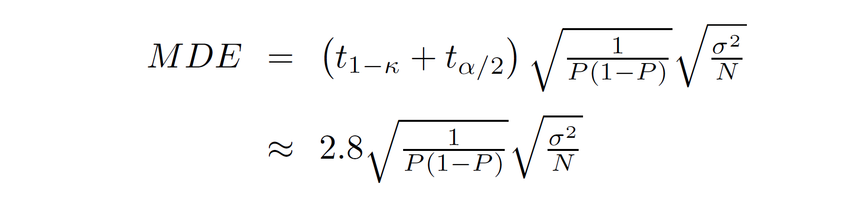
When we fix the size of the test at 0.05 and the power of the test at 0.8, the t_{1 - κ} + t_α/2 term is approximately equal to 2.8 (more on that in the next exercise). We also know that half of our sample is assigned to treatment, so P=0.5. Finally, we know that our outcome of interested is drawn from a standard normal distribution, so σ²=1. Given this, what is the minimum detectable effect when we use a sample of size 100? When you plug that MDE into the program as the value of the effect variable, you should see that you (correctly) reject the null hypothesis approximately 80 percent of the time. (Don’t forget to increase the sample size to 100!)

Question 13

Check that this is approximately correct by running the command

sampsi 0 0.56, power(0.8) sd(1)

which calculates the sample size required to have power 0.8 to test the hypothesis that treatment increases the mean from 0 to 0.56 when the SD of the outcome variable is 1. What is the total sample size required to conduct this hypothesis test (n1+n2)?